Chapter 2 Introduction
2.1 Linear models - a kind of Generalized Linear Model
If you have fit a linear model before, congratulations! You have already fit (one case) of a generalized linear model (GLM). Over the course of this book, we will explore the framework of Generalized Linear Models, why the Linear Model is a special case of a GLM, and two common type of GLMs, including logistic regression (for binary/binomial count data) and poisson regression (for count data).
Let’s review why we would fit a linear model. For linear regression, given our data, (if we make some key assumptions 2.2 ), we can perform inference or prediction by assuming that our response value forms a linear relationship with our explanatory variable (or variables). Generalized linear models expand upon the linear model assumptions to increase the kinds and ways we can use data to answer questions.
The reasoning behind linear models can be intuitive; if we have two continuous variables, and make a scatterplot our data, and see this:
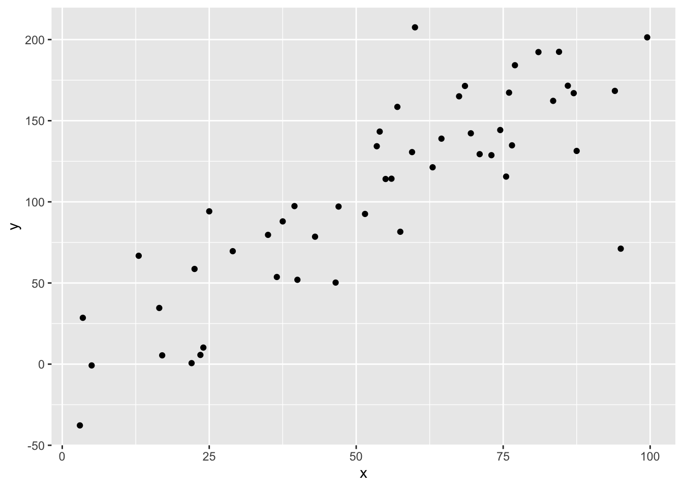
Figure 2.1: A scatterplot of points for two numeric variables.
We might want to fit a straight line through the cloud of points, i.e. modeling the relationship linearly.

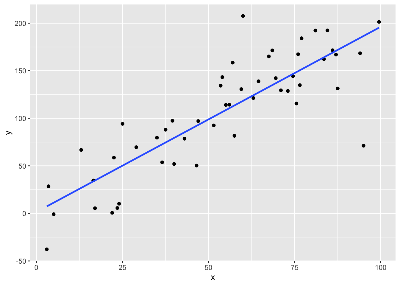
Figure 2.2: A scatterplot of points now with a line of best fit added.
To interpret this relationship and make predictions, we need to know the slope and intercept of this line. This is done by minimizing the least squares, which will be explored in Chapter 3 @ref{linear}. (will it? should it?) Linear models can also have multiple explanatory variables (\(X_1, \ldots X_p\) instead of just one \(X\)), and this becomes multiple linear regression. The visualization of this kind of data is more difficult, and for example purposes, we will only use one explanatory variable, \(X\).
2.2 Assumptions of Linear Models
A linear model might very well be a good model if we have data like that shown in Figures 2.1 and 2.2. However, there are many cases where it might be inappropriate to use a linear model. To understand these cases, we first review the assumptions of linear models.
Linear models assume:
- The relationship between the explanatory variables and the response is linear.
- The samples are independent.
- The errors are normally distributed with mean 0 and constant variance.
You might have seen these assumptions written in notation as such.
\[y_i = \beta_0 + \beta_1 x_i + \epsilon_i \] where \((x_i, y_i)\) represents the observed values for observation \(i = 1, 2, \ldots, n\) and \[ \epsilon_i \overset{\text{iid}}{\sim} N(0,\sigma^2)\]
In words, this means that the errors are independent and identically distributed from a normal distribution with mean 0 and constant variance \(\sigma^2\) (Notice how there is no subscript \(i\) for the variance. This means that all our our \(y_i\) values will have the same variation, regardless of what their associated values of \(x_i\) are). If we are performing multiple linear regression with up to \(p\) explanatory variables then this first assumption becomes \(y_i = \beta_0 + \beta_1 x_{1,i} + \ldots + \beta_p x_{p,i} + \epsilon_i\). That is, our response variable, \(Y\), is a linear function of the explanatory variables \(X_1, X_2, \ldots, X_p\).
2.3 Reframing Linear Models as Generalized Linear Models
To see how the linear model is just a special type of Generalized Linear Model, we will slightly modify how we think of these assumptions, so as to be able to more easily see the parallels. Instead of the response \(y_i\), now consider the mean response \(\mu_i\), which for a given value of one predictor \(x_i\) is the mean, or expected value of all responses with the value of that explanatory variable.
Then our assumptions become:
\[\begin{equation} \mu_i = \beta_0 + \beta_1 x_i \tag{2.1} \end{equation}\]
\[\begin{equation} y_i \overset{\text{iid}}{\sim} N(\mu_i, \sigma^2)\tag{2.2} \end{equation}\]
We refer to the first condition, Equation (2.1), as the Systematic Component and the second condition, Equation (2.2), as the Random Component. In this framework, the systematic component describes how the explanatory variables impact some parameter, in this case the mean. Once we model how the mean parameter changes depending on the explanatory variable, the random component then describes the variability we see in the response given the value of the parameter.
Generalized Linear Models are inspired by this idea of generalizing the random and systematic component of linear models. More broadly, a Generalized Regression Model has a systematic component
\[ g(\mu_i) = \beta_0 + \beta_1 x_i + \epsilon_i\]
where, in order to generalize the systematic component, we use a link function \(g(y)\) which then requires some function of the response to be linearly related to our explanatory variables.
The random component can then be written in general as:
\[y_i \overset{\text{iid}}{\sim} EDM(g(\mu_i), \phi) \]
Where EDM stands for a probability distribution from the Exponential Dispersion Family (EDM). We discuss these EDMs in greater detail in the next chapter but we can note for now that the Normal, Binomial, and Poisson distributions all belong to the Exponential Dispersion Family. The EDM distribution we use depends on the mean response, as well as a dispersion parameter \(\phi\). For many commonly use GLMs, and the ones discussed in this book, this \(\phi\) is known.
We note that normal linear models fall easily into this framework, where \(g(y_i) = y_i\) the identity function, and use the Normal distribution as our random component.
Deciding on what Random and Systematic component to use in a model requires …. us to have some idea about both the possible values our response variable takes as well as having some idea about which probability distribution might have generated our response.
2.4 What happens when we break the assumptions of linear models
How can we tell when these assumptions are violated? We can examine both the random and systematic component and see if our data can/should be modeled in such a way. This largely comes from knowledge of the data.
Linear models are generally robust, and can be reasonable when assumptions are not exactly met. However, if we know assumptions are not met, and how they are not met, it is appropriate to use a more appropriate model for the data.
2.5 Parameter estimation
Another difference between linear models and generalized linear models is the way we estimate the parameters \(\beta\). For linear models, we find the minimize the sums of squares from the predictor to the response(s). This has a closed form solution, and can be calculated by hand (if one really wanted to). For generalized linear models, we estimate the \(\beta\) parameters using Maximum Likelihood Estimation. For the Normal linear model case, this is equivalent to minimizing the sums of squares. However, for other GLMs, there is no closed form solution, which requires us to perform an iterative algorithm to land at the parameter estimates. Luckily this is all done behind the scenes in R. Those interested in learning more about how parameter estimation works for GLMs can read Chapter 6 of (Dunn and Smyth 2018).
2.6 LMs and GLMs in R
Fitting GLMs in R is very similar to fitting linear models in R. For linear models, we use the function lm(). For generalized regression models, we use the function glm(). Both require a formula input, but glm() also requires the user to specify the random and systematic part of a GLM, by specifying the family and link function. Help for fitting a GLM can be found by ?glm() and reading more about the family argument.
Let’s use some simulated data to see how GLMs are fit in R, and
##           y     x1    x2
## 1 -428.3313 225.50 299.7
## 2 -450.6219 203.75 292.9
## 3 -490.0964 107.75 221.0
## 4 -396.5941  93.50 202.1
## 5 -355.2111 246.50 287.2
## 6 -320.0738 212.00 260.6
First, fit a linear model the normal way, using lm()
##
## Call:
## lm(formula = y ~ x1 + x2, data = sim_data)
##
## Residuals:
##     Min      1Q  Median      3Q     Max
## -45.374 -12.734   1.415  14.029  50.782
##
## Coefficients:
##             Estimate Std. Error t value Pr(>|t|)
## (Intercept) -9.34841   18.70405   -0.50    0.619
## x1           2.03291    0.02354   86.34   <2e-16 ***
## x2          -2.96118    0.07611  -38.90   <2e-16 ***
## ---
## Signif. codes:  0 '***' 0.001 '**' 0.01 '*' 0.05 '.' 0.1 ' ' 1
##
## Residual standard error: 20.15 on 72 degrees of freedom
## Multiple R-squared:  0.9912, Adjusted R-squared:  0.991
## F-statistic:  4062 on 2 and 72 DF,  p-value: < 2.2e-16
Now we show that we can use glm() the same way, specifying family = "gaussian", which gives the identity link.
##
## Call:
## glm(formula = y ~ x1 + x2, family = "gaussian", data = sim_data)
##
## Deviance Residuals:
##     Min       1Q   Median       3Q      Max
## -45.374  -12.734    1.415   14.029   50.782
##
## Coefficients:
##             Estimate Std. Error t value Pr(>|t|)
## (Intercept) -9.34841   18.70405   -0.50    0.619
## x1           2.03291    0.02354   86.34   <2e-16 ***
## x2          -2.96118    0.07611  -38.90   <2e-16 ***
## ---
## Signif. codes:  0 '***' 0.001 '**' 0.01 '*' 0.05 '.' 0.1 ' ' 1
##
## (Dispersion parameter for gaussian family taken to be 405.8226)
##
##     Null deviance: 3326225  on 74  degrees of freedom
## Residual deviance:   29219  on 72  degrees of freedom
## AIC: 668.22
##
## Number of Fisher Scoring iterations: 2
As you can see from the summary outputs, we get results which are very similar, as we should, since both functions fit the same model. However, some outputs of our linear model are slightly different when we compare them to the GLM version. For instance, we no longer have values for the residual standard errors, R-squared values and F-statistics. Instead, in the GLM, we have summary values like the null and residual deviance along with the AIC. We’ll talk more about these differences in future chapters. But for now, know that many of the functions we used for linear models, like coef(), predict(), etc, will perform as expected, when we pass a generalized linear model fitted using glm() in as the first argument.
2.7 Some definitions
We close this chapter with some definitions of common terminology and explanation of notation that will be used throughout this text.
Predictor - the thing on the y-axis Explanatory variable - the stuff on the x-axis. Note that we can have more than one (but won’t plot it then), and then this becomes multiple variable regression.
Something that is an estimated quantity will have a hat over it. For example, we might assume that there is some ‘true’ (but unknown) linear relationship between our explanatory variables and our predictor.
\[ y = \beta_0 + \beta_1 x\]
From our sample data, we use a linear model to make an estimate of \(\beta_0\) and \(\beta_1\),
so our estimate/best guess of this true model relationship is
\[ \hat y = \hat\beta_0 + \hat\beta_1 x\] We of course want our \(\hat\beta_0\) and \(\hat\beta_1\) to be a ‘good’ and ‘close’ estimate of the unknown quantities \(\beta_0\) and \(\beta_1\). Ideas of what ‘good’ and ‘close’ mean will be covered in the next section.
2.8 Conclusion
Linear models are not always the best tool for describing relationship in data. Luckily we can generalize the ideas and framework developed in linear models to hold for more general cases to create GLMs. Using a more general framework and more general assumptions allows us to build tools that will hold for all GRMs. The most notable of these that we will further explore are GRMs for binary data (ch4) and count data (ch5)
2.9 Examples
Perhaps some examples of data and students can tell what type of data it should be modeled by?
Explore the following case of where a linear model is NOT appropriate, and then fit a glm() call in R using an appropriate family and link function.
Note that this example might take a minute to load.
References
Dunn, Peter K, and Gordon K Smyth. 2018. Generalized Linear Models with Examples in R. Springer.